Tutorial 06: Collect Across Time

Collecting and examining data collected across time.

Collecting By Time

The EUtils API allows for selecting a date range to collect articles published within particular time frames. One thing we can use this for is to collect information for articles published across time.

# Import LISC objects
from lisc import Counts1D, Words

# Import function to collect literature data over time
from lisc.collect import collect_across_time

# Import plots that are available for time-related analyses
from lisc.plts.time import plot_results_across_years

Example 1: Simple Example of Counts over Years

In this first example, we will use the Counts1D class and approach to collect information about how many papers discuss a topic over time.

To do so, we will first define a simple set of terms, and initialize the LISC object.

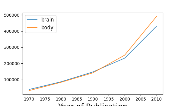
# Define a set of terms to use
terms_a = ['brain', 'body']

# Initialize a Counts1D object to use
counts = Counts1D()

# Add terms to counts object
counts.add_terms(terms_a)

Next we have to define the time range(s) that we want to collect literature data for!

To do so, we define a list of years which specifies a set of ranges to collect data for.

By default, all date ranges reflect full years, from January 1st of the start year until December 31st of the year prior to the listed end year (so that there is no overlap).

For example, if a list of years was defined [1900, 1950, 2000], this would collect data for:

• year range 1900-1950, defined as January 1st 1900 to December 31st 1949

• year range 1950-2000, defined as January 1st 1950 to December 31st 1999

# Define a range of years to collect data for
years_a = [1970, 1980, 1990, 2000, 2010, 2020]

To run a collection of literature data across time, we use the collect_across_time() function.

This function takes as input a pre-initialized LISC object, used to collect the data, as well as the definition of which years to run the search for.

# Collect counts data across years
year_results = collect_across_time(counts, years_a)

Running this collection returns a list of LISC objects, which each object corresponding to a time range as defined by the years argument.

# Check the output of running the collection across time
year_results

{1970: <lisc.objects.counts.Counts1D object at 0x7f85bfd8ea00>, 1980: <lisc.objects.counts.Counts1D object at 0x7f85bfd8e3d0>, 1990: <lisc.objects.counts.Counts1D object at 0x7f85bf0bec40>, 2000: <lisc.objects.counts.Counts1D object at 0x7f85bf0be070>, 2010: <lisc.objects.counts.Counts1D object at 0x7f85bf0be3a0>}

Now that we have collected this data

For example, if collecting Counts data as done here, the plot_results_across_years() function can be used to plot the results across the collected time ranges.

# Plot the results over time
plot_results_across_years(year_results)

Example 2: Additional Counts Explorations

In the first example, we searched for simple term counts across time. Searches across time also support more complex terms and search criteria.

In this example, we will search for a more complex counts analysis across time.

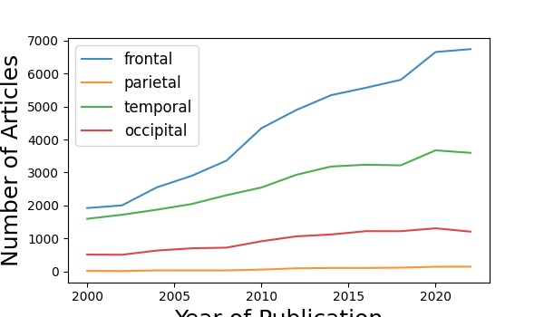
# Define range of years to collect data for
years_b = list(range(2000, 2026, 2))

# Define terms lists
terms_b = ['frontal', 'parietal', 'temporal', 'occipital']
inclusions_b = ['brain', 'neuroscience', 'lobe', 'cortex']

# Initialize LISC object and add terms
counts = Counts1D()
counts.add_terms(terms_b)
counts.add_terms(inclusions_b, 'inclusions')

# Run collection across time
year_results = collect_across_time(counts, years_b)

As before, the output of collect_across_time is a list of returned LISC objects.

We can examine the results for a particular time period.

# Access an individual search
year_results[2010].check_counts()

The number of documents found for each search term is:
  'frontal'     -   4341
  'parietal'    -     56
  'temporal'    -   2544
  'occipital'   -    915

We can also plot the results across years, comparing across all search items.

# Plot the results over time
plot_results_across_years(year_results)

Example 3: Words

In the examples above, we searched for article counts and co-occurrences across time, We can also collect article information across time, using the Words object.

To do so, as before we start by defining the time range to search, and our search terms.

# Define time ranges to collect data across
decades = [1930, 1940, 1950]

# Define search terms
terms_c = ['metabolism']
incl_c = ['brain']

Now we can add our search terms to a Words object.

# Initialize words object, and add terms
words = Words()
words.add_terms(terms_c)

Next, we pass in the pre-initialized Words object to the collect_across_time, also passing in any word collection settings.

# Word collection settings
retmax = 5

# Collect words results across time
word_results = collect_across_time(words, decades, retmax=retmax)

As before, the output is a list of LISC objects, each containing the results for a particular time period.

We can loop across these objects to examines results per time period.

# Check the titles found across different time ranges
for time_period, results in word_results.items():
    print(str(time_period) + 's:')
    for res_title in results.results[0].titles:
        print('\t', res_title)

1930s:
         A DEFECT IN THE METABOLISM OF AROMATIC AMINO ACIDS IN PREMATURE INFANTS: THE ROLE OF VITAMIN C.
         Metabolism of the Heart.
         The metabolism of normal and tumour tissue: The action of guanidines and amidines on the Pasteur effect.
         The role of sorbitol in the C-metabolism of the Kelsey plum: Relation of carbohydrate and acid loss to CO(2) production in stored fruit.
         THE METABOLISM OF GLUTATHIONE.
1940s:
         [Carbohydrate metabolism disorders in the course of minor chronic diarrhea].
         The low metabolic state.
         Iron metabolism in liver disease.
         [Effect of histidine on glucide metabolism].
         Action of potassium ions on brain metabolism.

That completes the tutorial for searching across time!