Tutorial 04: Counts Analysis

Analyzing collected co-occurrence data.

Counts Analyses

This tutorial explores analyzing collected co-occurrence data.

Note that this tutorials requires some optional dependencies, including matplotlib, seaborn and scipy.

# Import database and IO utilities to reload our previously collected data
from lisc.io import SCDB, load_object

# Import plots that are available for co-occurrence analysis
from lisc.plts.counts import plot_matrix, plot_clustermap, plot_dendrogram

# Reload the counts object from the last tutorial
counts = load_object('tutorial_counts', SCDB('lisc_db'))

The Counts object has some helper methods to explore the collected data.

First lets check the number of counts per term list, which we can do with the check_data() method.

# Look at the collected counts data for the first set of terms
counts.check_data(data_type='counts', dim='A')

For  'frontal lobe'    the highest association is  'audition'        with         459
For  'temporal lobe'   the highest association is  'audition'        with        1543
For  'parietal lobe'   the highest association is  'audition'        with         275
For  'occipital lobe'  the highest association is  'vision'          with         303

# Look at the collected counts data for the second set of terms
counts.check_data(data_type='counts', dim='B')

For  'vision'          the highest association is  'occipital lobe'  with         303
For  'audition'        the highest association is  'temporal lobe'   with        1543
For  'somatosensory'   the highest association is  'temporal lobe'   with         223
For  'olfaction'       the highest association is  'temporal lobe'   with          96
For  'gustation'       the highest association is  'temporal lobe'   with          54
For  'proprioception'  the highest association is  'parietal lobe'   with          12
For  'nociception'     the highest association is  'temporal lobe'   with         271

Normalization & Scores

The collected co-occurrence data includes information on the number of articles in which terms co-occur, as well as the number of articles for each term independently.

Once we have this data, we typically want to calculate a normalized measures, and/or other kinds of similarity score, to compare between terms.

To normalize the data, we can divide the co-occurrence counts by the number of articles per term. This allows us the examine, for example, the proportion of articles that include particular co-occurrence patterns.

These measures are available using the compute_score() method. This method can compute different types of scores, with the type specified by the first input to the method. Scores available include ‘normalize’, ‘association’, or ‘similarity’.

# Compute a normalization of the co-occurrence data
counts.compute_score('normalize', dim='A')

# Check out the computed normalization
print(counts.score)

[[1.17668248e-02 2.75559825e-02 9.30539713e-03 4.14240259e-03
  1.20069640e-03 2.40139281e-04 1.33277301e-02]
 [7.40606390e-03 4.66430882e-02 6.74102959e-03 2.90196790e-03
  1.63235694e-03 6.04576645e-05 8.19201354e-03]
 [1.75409836e-02 4.50819672e-02 3.52459016e-02 1.47540984e-03
  1.47540984e-03 1.96721311e-03 2.47540984e-02]
 [6.53017241e-02 2.43534483e-02 1.07758621e-02 1.07758621e-03
  0.00000000e+00 2.15517241e-04 1.85344828e-02]]

The normalization is the number of articles with both terms, divided by the number of articles for a single term. It can therefore be interpreted as a proportion of articles with term a that also have term b, or as a & b / a.

Note that when using two different terms lists, you have to choose which list of terms to normalize by, which is controlled by the dim input.

In this case, we have calculated the normalized data as the proportion of articles for each anatomical term that include each perception term.

Alternately, we can also calculate an association index or score, as below:

# Compute the association index
counts.compute_score('association')

# Check out the computed score
print(counts.score)

[[1.13145028e-03 3.40749649e-03 3.02568908e-03 1.91592159e-03
  3.57980275e-04 1.71629623e-04 2.74766418e-04]
 [1.29216683e-03 1.02837187e-02 3.29959754e-03 1.83167656e-03
  7.47311754e-04 5.03372596e-05 3.28750240e-04]
 [6.57405644e-04 2.21185555e-03 5.29413213e-03 3.52706039e-04
  1.98574675e-04 9.41841300e-04 1.89348103e-04]
 [1.88076099e-03 9.18460238e-04 1.27174687e-03 2.07805162e-04
  0.00000000e+00 8.85582713e-05 1.08029615e-04]]

Specifying ‘association’ computes the Jaccard index, which is a standard measure for measuring the similarity of samples, calculating a normalized measure of similarity, bounded between 0 and 1.

One benefit of the Jaccard index is that you do not have to choose a terms list to normalize by - the calculated measure considers both lists of terms to compute an association index.

The cosine similarity of the co-occurrence data can also be calculated, with ‘similarity’.

Clustering and Plotting Co-occurrence Data

The collected co-occurrence data is a 2D matrix of counts reflecting the relationship between terms. This makes it amenable to visualizations and analyses, such as clustering, that look to find structure in the data.

LISC provides some functions to visualize and cluster co-occurrence data. These functions use functionality offered by optional dependencies, including scipy and seaborn, which need to be installed for these to run.

The functions plot_matrix(), plot_clustermap(), and plot_dendrogram() offer visualizations and clustering. You can check through each function for details on what each one is doing.

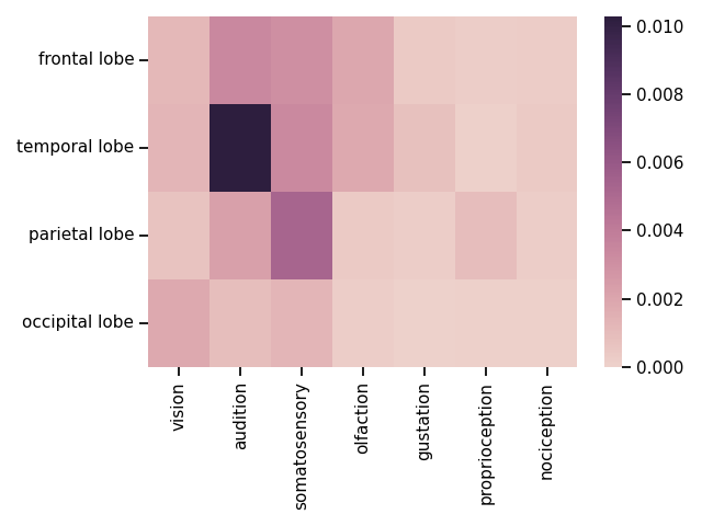
# Plot a matrix of the association index data
plot_matrix(counts, attribute='score')

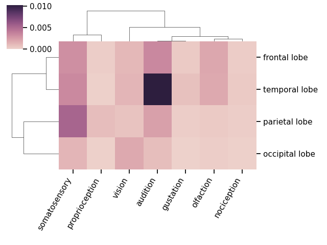
# Plot a clustermap of the association index data
plot_clustermap(counts, attribute='score')

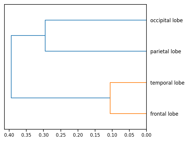
# Plot a dendrogram, to cluster the terms
plot_dendrogram(counts, attribute='score')